Normal Distribution

Schwab

Read before lecture

Open Intro Statistics 4.1 Normal Distribution

Normal Distribution

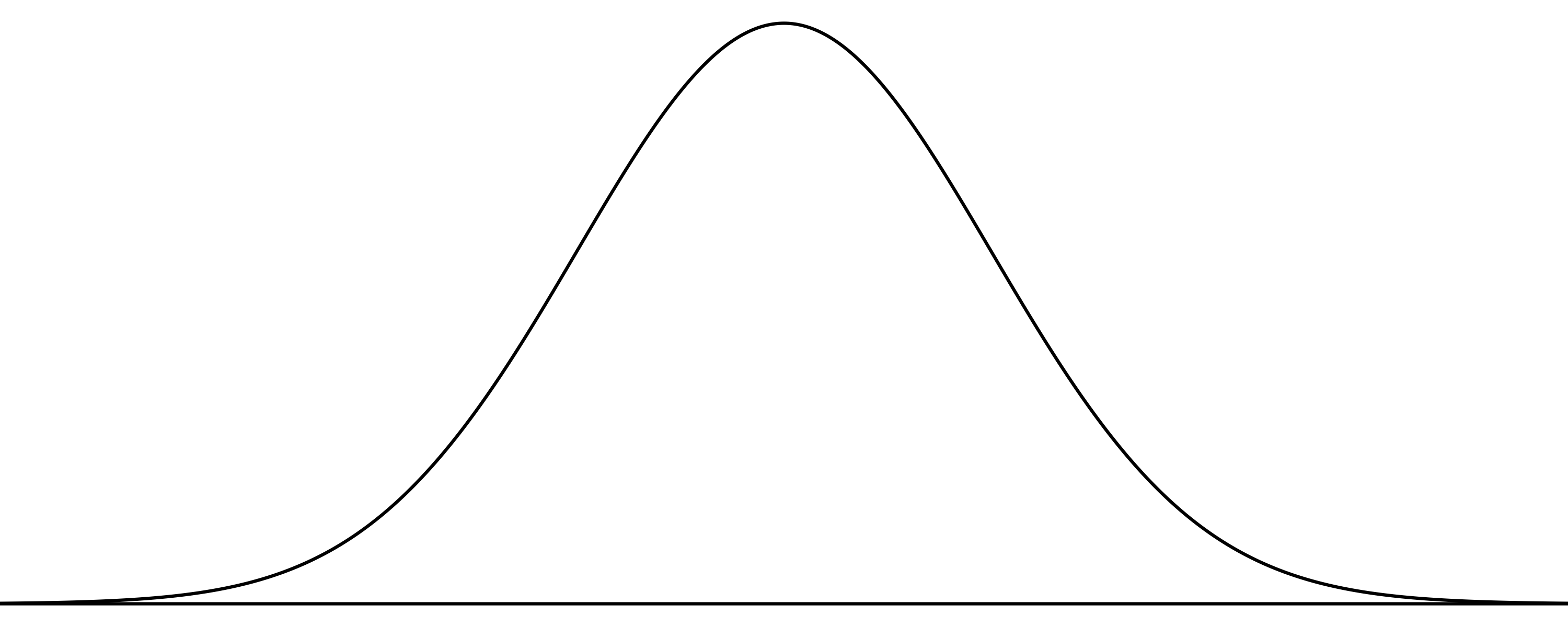
The normal distribution has a symmetric bell shaped curve

library(openintro)
normTail()

The picture above is for the so called standard normal distribution.

The Standard Normal

Has a mean \(\mu = 0\) and standard deviation \(\sigma = 1\)

Notation \(X\sim N(\mu,\sigma)\) means the random variable X has a normal distribution.

It is what z-scores are based on. (There are other distributions).

Very Short history lesson.

• Long long ago before computers existed people wanted to calculate probabilities from z-scores.

• The table was first made by Christian Kramp in 1799.

• It was improved upon ( for more read this).

• We will not use the ancient table

Brushtail possum

Problem from text:

Head lengths of brushtail possums follow a nearly normal distribution (it is also a continuous random variable) with mean 92.6 mm and standard deviation 3.6 mm. Compute the [percentiles] for possums with head lengths of 95.4 mm and 85.8 mm.

Which of the two brushtail possum observations in the previous guided practice is more unusual?

Picture the distribution

\(X \sim N(\mu = 92.6 , \sigma = 3.6)\)

normTail(m=92.6,s=3.6)

The graph for the first possum

normTail(m=92.6,s=3.6, L = 95.4)

The graph for the second possum

normTail(m=92.6,s=3.6, L = 85.8)

Calculate percentiles with R

We use pnorm() to find percentiles.

pnorm(q=85.8 ,m = 92.6, s = 3.6 )

[1] 0.02945336

This finds the probability to the left of q.

pnorm(q=85.8 ,m = 92.6, s = 3.6, lower.tail = FALSE)

[1] 0.9705466

Visualize with openintro package

library(tidyverse)
library(openintro)

pnorm(q=85.8 ,m = 92.6, s = 3.6, lower.tail = FALSE )

[1] 0.9705466

normTail(m = 92.6, s= 3.6, U = 85.8)

Calculus

The function f(x) below defines the pdf of the bell curve.

\[ f(x) = \frac{1}{\sigma \sqrt{2 \pi}} e^{-\frac{1}{2}(\frac{x-\mu}{\sigma})^2 } \]

What we really care about:

The probability is the area under the curve and can be represented as:

\[ \int_a^b \frac{1}{\sigma \sqrt{2 \pi}} e^{-\frac{1}{2}(\frac{x-\mu}{\sigma})^2 } dx \]

We will not be computing these values by hand.

Reminder:

Draw the curve and the integral that goes with the possum area under the normal distribution.

The Empirical rule.

Draw a picture of the standard normal bell curve. Mark -1 and 1 \(\sigma\) away from the mean.

Using R find the probability we get values between -1 and 1. shade your picture.

Repeat this process for [-2,2] and [-3,3].

Practice

From the text:

SAT scores closely follow the normal model with mean μ=1500 and standard deviation σ=300. About what percent of test takers score 900 to 2100? What percent score between 1500 and 2100

Practice 2

Shannon is a randomly selected SAT taker, and nothing is known about Shannon’s SAT aptitude. What is the probability that Shannon scores at least 1630 on their SATs?

Practice 3

Edward earned a 1400 on their SAT. What is their percentile?

What percent did better than Edward?

qnorm outputs quantiles from percents.

#|echo: TRUE

pnorm(q = 85.8 ,m = 92.6, s = 3.6 )

[1] 0.02945336

qnorm(p = 0.02945336, m = 92.6, s = 3.6)

[1] 85.8

qnorm() is for finding quantiles pnorm() is for finding percentiles.

Practice 4

OI 4.2 d

Compute the mean and sd

Note on notation.

\(X \sim N(\mu = 92.6 , \sigma = 3.6)\)

or

\(X \sim N(\bar{x} = 92.6 , s= 3.6)\)
We estimate \(\sigma\) with s - The sample proportion.

# Sample standard deviation

sd(possum$head_l)

[1] 3.573349

# Sample mean
mean(possum$head_l, na.rm = TRUE)

[1] 92.60288