Taxonomy of Graphs part 1: Categorical

CSI-MTH-190

Schwab

PreReqs

I assume you’ve read chapter 2.2, if you haven’t, go back and read it before this lecture.

The Data

In this lecture I’ll use one set of data called starwars to illustrate some of the ideas you should consider when building a graph.

We’ll focus mostly on the categorical variables in this lecture. Next week we’ll tackle the numeric variables.

library(tidyverse)
library(mdsr)
head(starwars)

# A tibble: 6 × 14
  name      height  mass hair_color skin_color eye_color birth_year sex   gender
  <chr>      <int> <dbl> <chr>      <chr>      <chr>          <dbl> <chr> <chr> 
1 Luke Sky…    172    77 blond      fair       blue            19   male  mascu…
2 C-3PO        167    75 <NA>       gold       yellow         112   none  mascu…
3 R2-D2         96    32 <NA>       white, bl… red             33   none  mascu…
4 Darth Va…    202   136 none       white      yellow          41.9 male  mascu…
5 Leia Org…    150    49 brown      light      brown           19   fema… femin…
6 Owen Lars    178   120 brown, gr… light      blue            52   male  mascu…
# ℹ 5 more variables: homeworld <chr>, species <chr>, films <list>,
#   vehicles <list>, starships <list>

Visual Cues Length

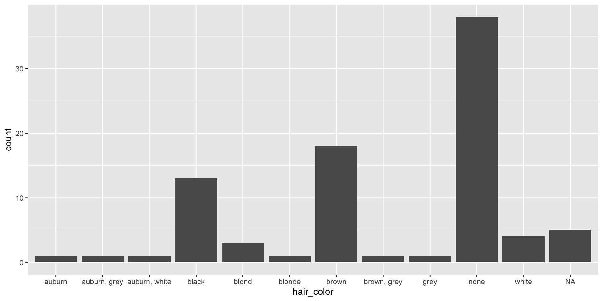
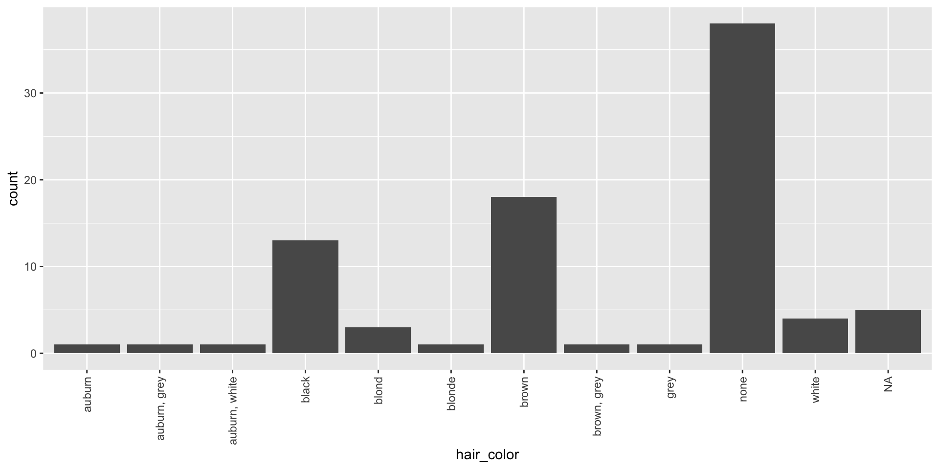
Show length with a bar chart

starwars |>
    ggplot()+
    geom_bar(aes(x=hair_color))

Visual Cues Length again

Show length with a bar chart

starwars |>
    ggplot()+
    geom_bar(aes(x=hair_color))+
    theme(axis.text.x = element_text(angle = 90, hjust = 1, vjust = 0.5))

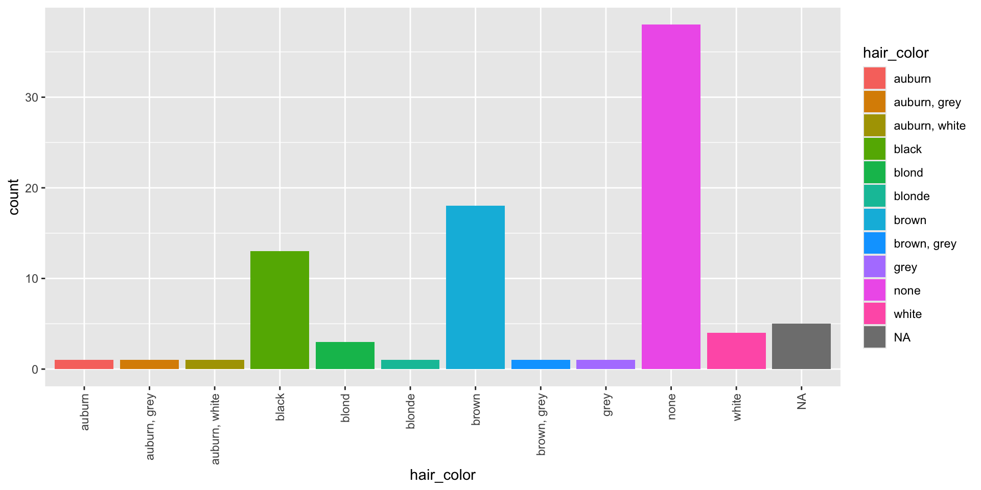
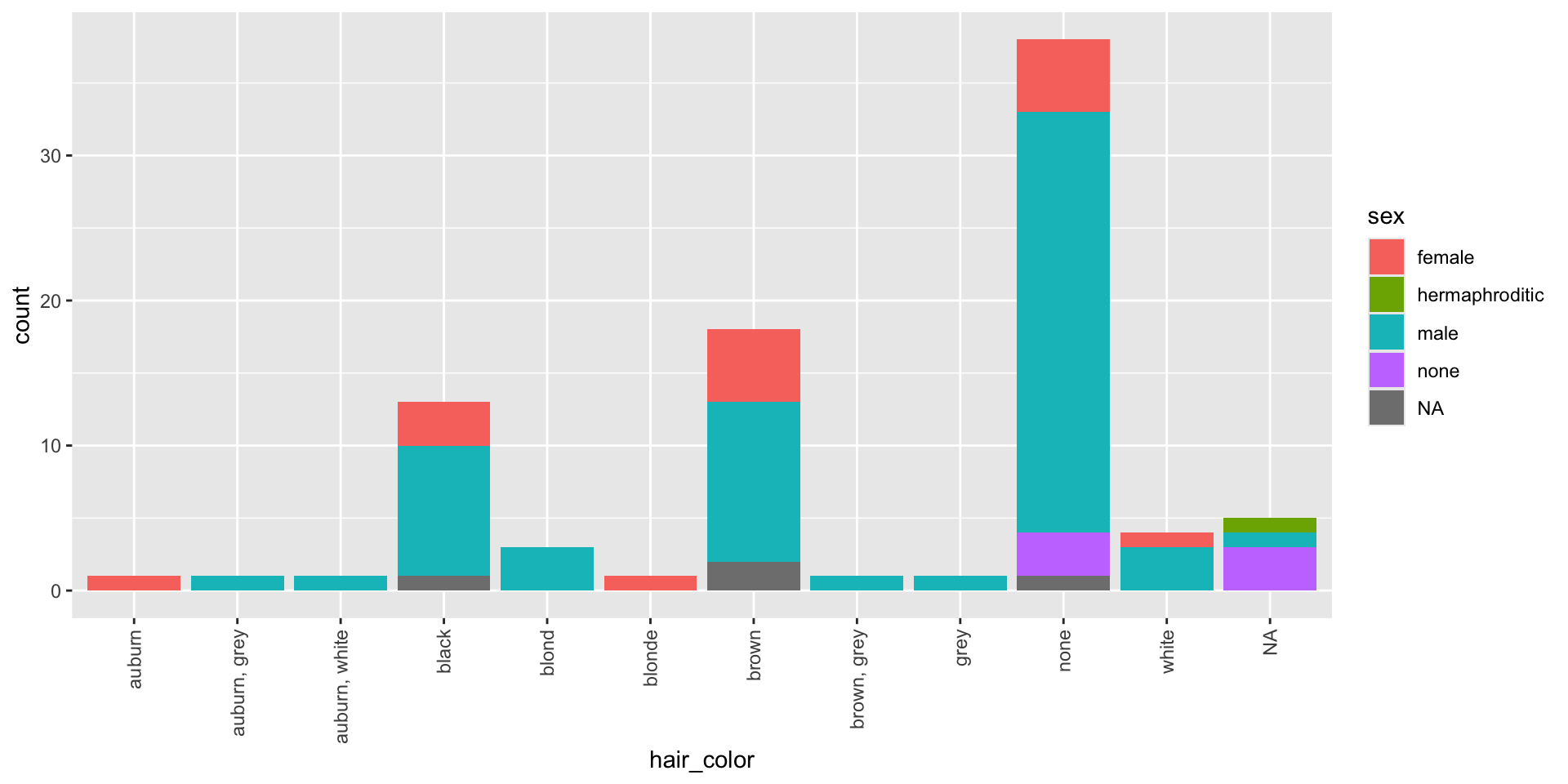
Visual Cues Color

Too many colors are not helpful. Below I fill each rectangle by hair_color.

And we now have a redundant mapping.

starwars |>
    ggplot()+
    geom_bar(aes(x=hair_color, fill = hair_color))+
    theme(axis.text.x = element_text(angle = 90, hjust = 1, vjust = 0.5))

Visual Cues Color again

Limit your colors to show another variable. Here I’ll fill by sex.

starwars |>
    ggplot()+
    geom_bar(aes(x=hair_color, fill = sex))+
    theme(axis.text.x = element_text(angle = 90, hjust = 1, vjust = 0.5))

You try:

Take a moment and copy the code below into r, fill by eye_color. What do you think about the graph?

starwars |>
    ggplot()+
    geom_bar(aes(x=hair_color ))+
    theme(axis.text.x = element_text(angle = 90, hjust = 1, vjust = 0.5))

Visual Cues Scale

In the graph below the scale is categorical on the x-axis and numeric on the y-axis.

starwars |>
    ggplot()+
    geom_bar(aes(x=hair_color, fill = sex))+
    theme(axis.text.x = element_text(angle = 90, hjust = 1, vjust = 0.5))

Visual Cues Context

Here I add a title, x and y axes and a source of the data.

starwars |>
    ggplot()+
    geom_bar(aes(x=hair_color, fill = sex))+
    labs(x = "Hair Color",
        y = "number of characters",
        title = "Hair Color of Starwars Characters",
        caption = "data from dplyr r package")+
    theme(axis.text.x = element_text(angle = 90, hjust = 1, vjust = 0.5))

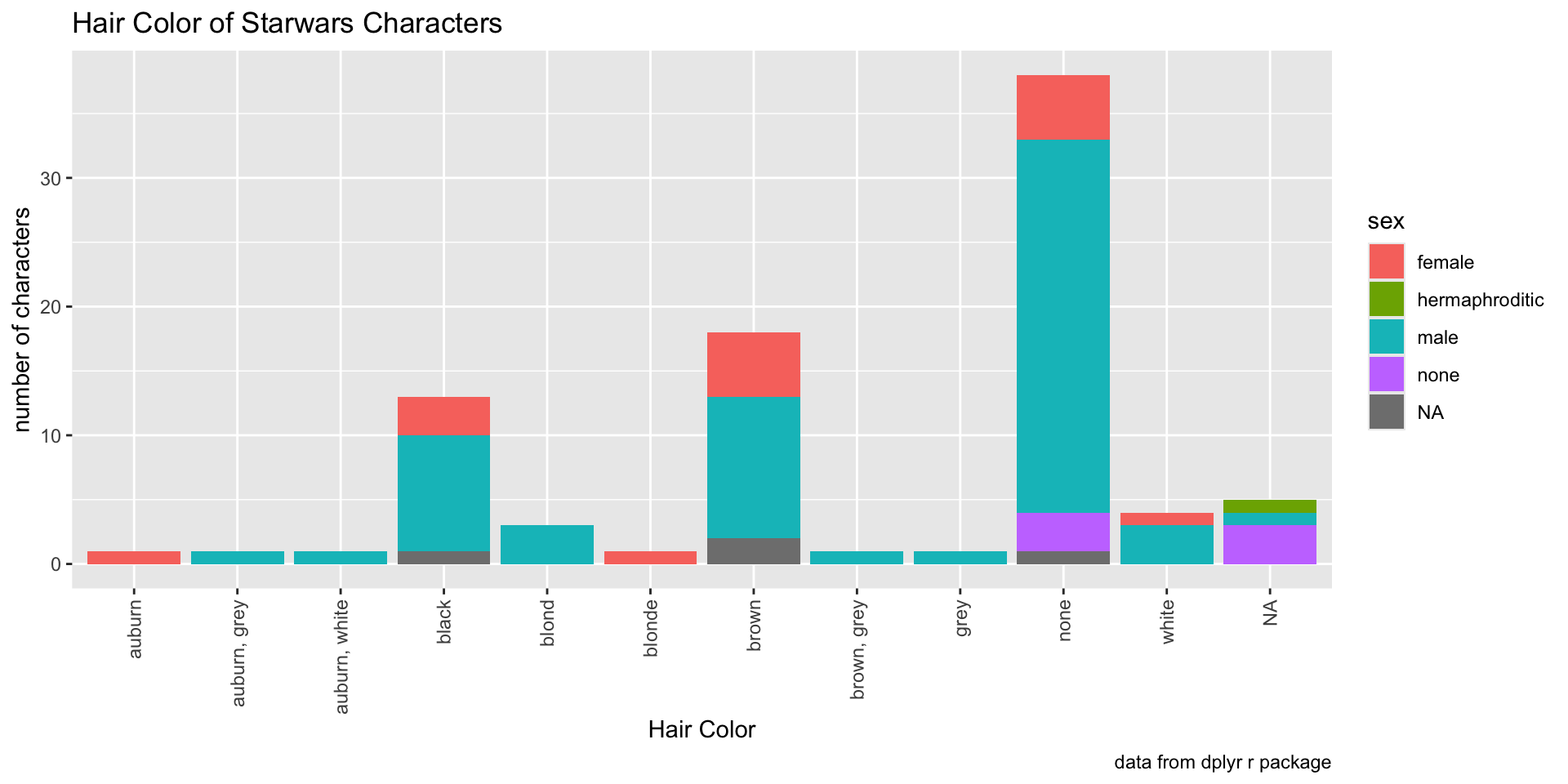
Touch ups

You can add a theme to the graph to easily make things look more professional. Pick your favorite theme and go with it.

Also I eliminated the x-axis label as it was redundant with the title.

starwars |>
    ggplot()+
    geom_bar(aes(x=hair_color, fill = sex))+
    labs(x = "Hair Color",
        y = "number of characters",
        title = "Hair Color of Starwars Characters",
        caption = "data from dplyr r package")+
    theme_mdsr()+
    theme(axis.text.x = element_text(angle = 90, hjust = 1, vjust = 0.5))