Taxonomy of Graphs part 2: Numeric Data

CSI-MTH-190

Schwab

Libraries

You may not have palmerpenguins installed. You’ll know if you get the following message:

Error in `library()`:

! there is no package called ‘palmerpenguins’

If so paste the install line into the console and type return/enter. (Remove the #).

library(tidyverse)
#install.packages("palmerpenguins")
library(palmerpenguins)

The Data

In this lecture I’ll use one set of data called palmerpenguins to illustrate some of the ideas you should consider when building a graph.

We’ll focus mostly on the numeric variables in this lecture, although many of the ideas are similar for both numeric and categorical variables.

Example mass

Recall how we can use summarize from lab 2 to calculate descriptive statistics.

# Putting inside of summarize is helpful
penguins |> 
  summarize(
    body_mass = mean( body_mass_g, na.rm=TRUE)
)

# A tibble: 1 × 1
  body_mass
      <dbl>
1     4202.

Below we can calculate the mean() with base R (i.e. without summarize()).

# But not necessary

mean(penguins$body_mass_g, na.rm = TRUE)

[1] 4201.754

Try one:

Find the median flipper length using summarize().

Answer:

To find the median flipper length using summarize() you would use this code in a chunk:

# Putting inside of summarize is helpful
penguins |> 
  summarize(
    body_mass = median( flipper_length_mm, na.rm=TRUE)
)

# A tibble: 1 × 1
  body_mass
      <dbl>
1       197

Boxplots

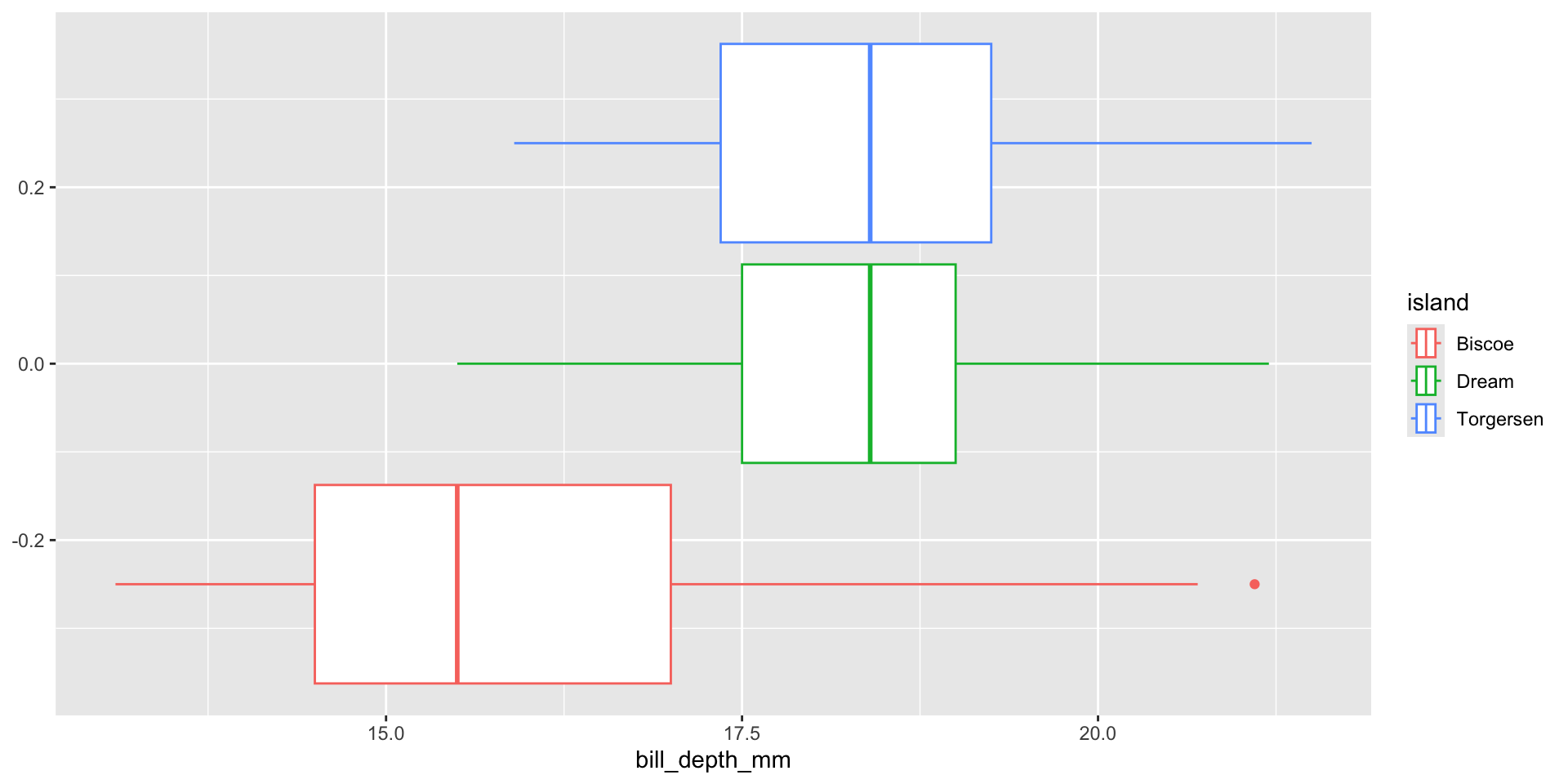
Boxplots are helpful for finding outliers.

Try to make a boxplot of the penguins bill_depth_mm color it by island.

Code for graph

## boxplot for bill depth, separated by island.

penguins |>
  ggplot(aes(x = bill_depth_mm, color = island))+
  geom_boxplot()

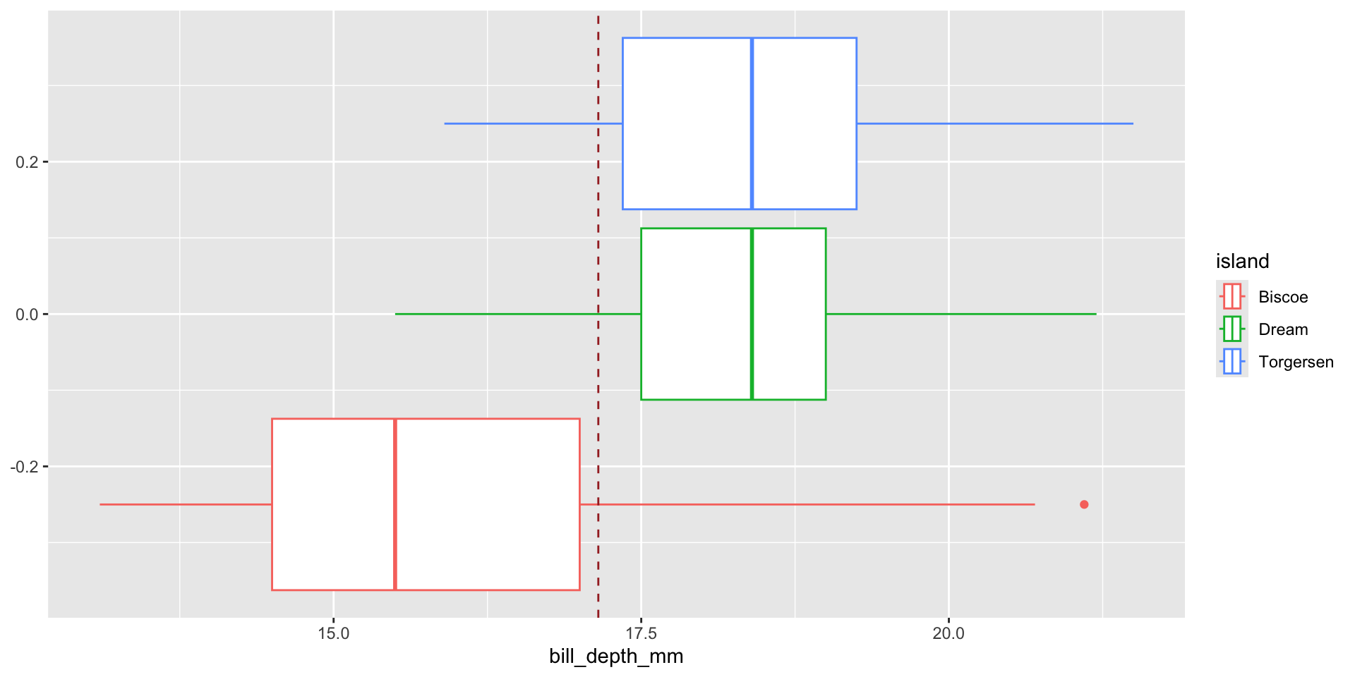
geom_vline()

If you want to mark part of the graph, sometimes a vertical line is helpful. You simply add on a geom_vline() layer.

# Adding a brown line to show the mean billdepth. 

mean_bill_depth = mean(penguins$bill_depth_mm, na.rm = TRUE)

penguins |>
  ggplot(aes(x = bill_depth_mm, color = island))+
  geom_boxplot()+
  geom_vline(
    xintercept = mean_bill_depth,
    color="brown",
    linetype="dashed")

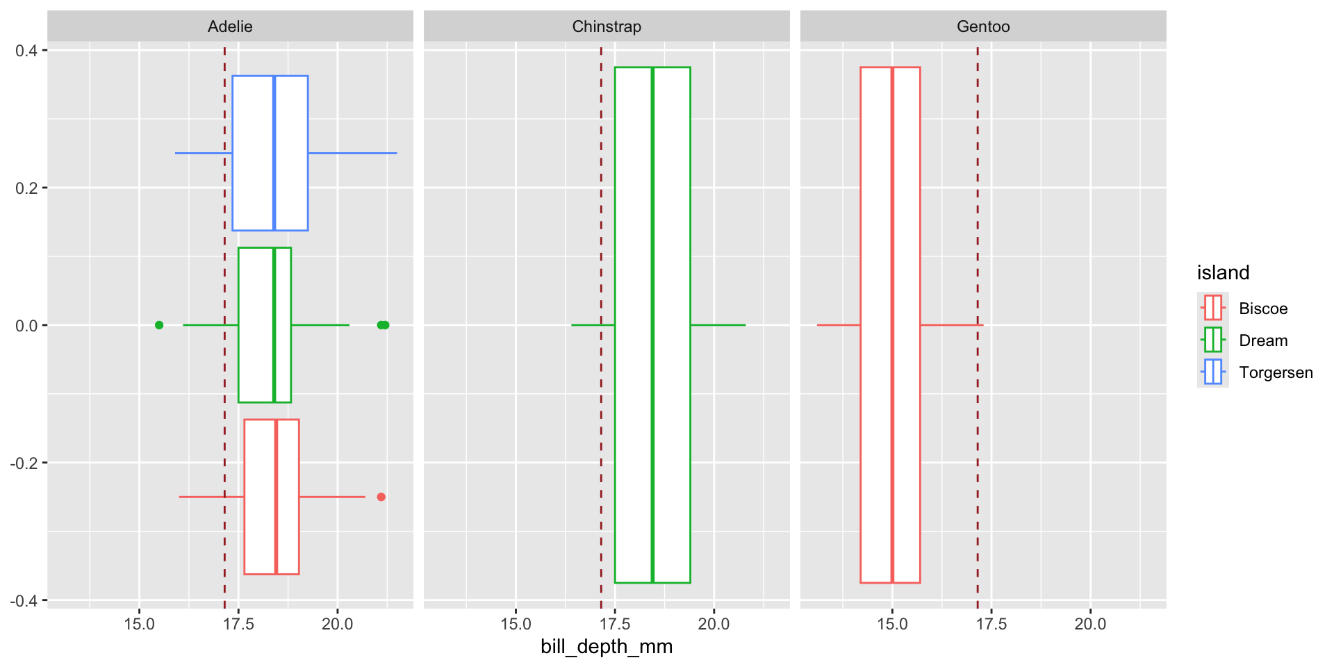
faceted

We can break code into smaller piece called facets.

# In the code below I am faceting by species

penguins |>
  ggplot(aes(x = bill_depth_mm, color = island))+
  geom_boxplot()+
  geom_vline(
    xintercept = mean(
      penguins$bill_depth_mm, na.rm = TRUE),
    color="brown",
    linetype="dashed")+
  facet_grid(~species)

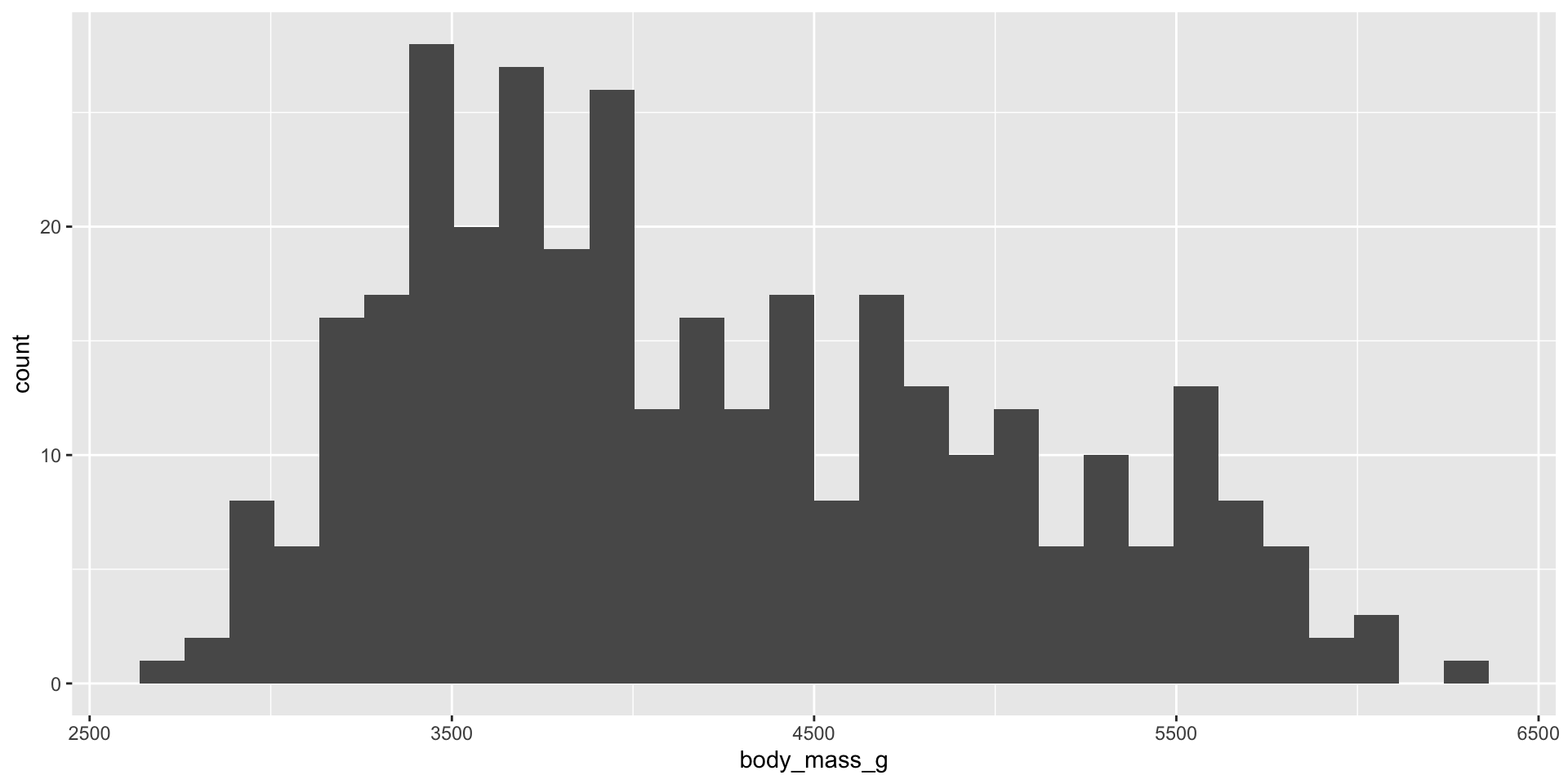
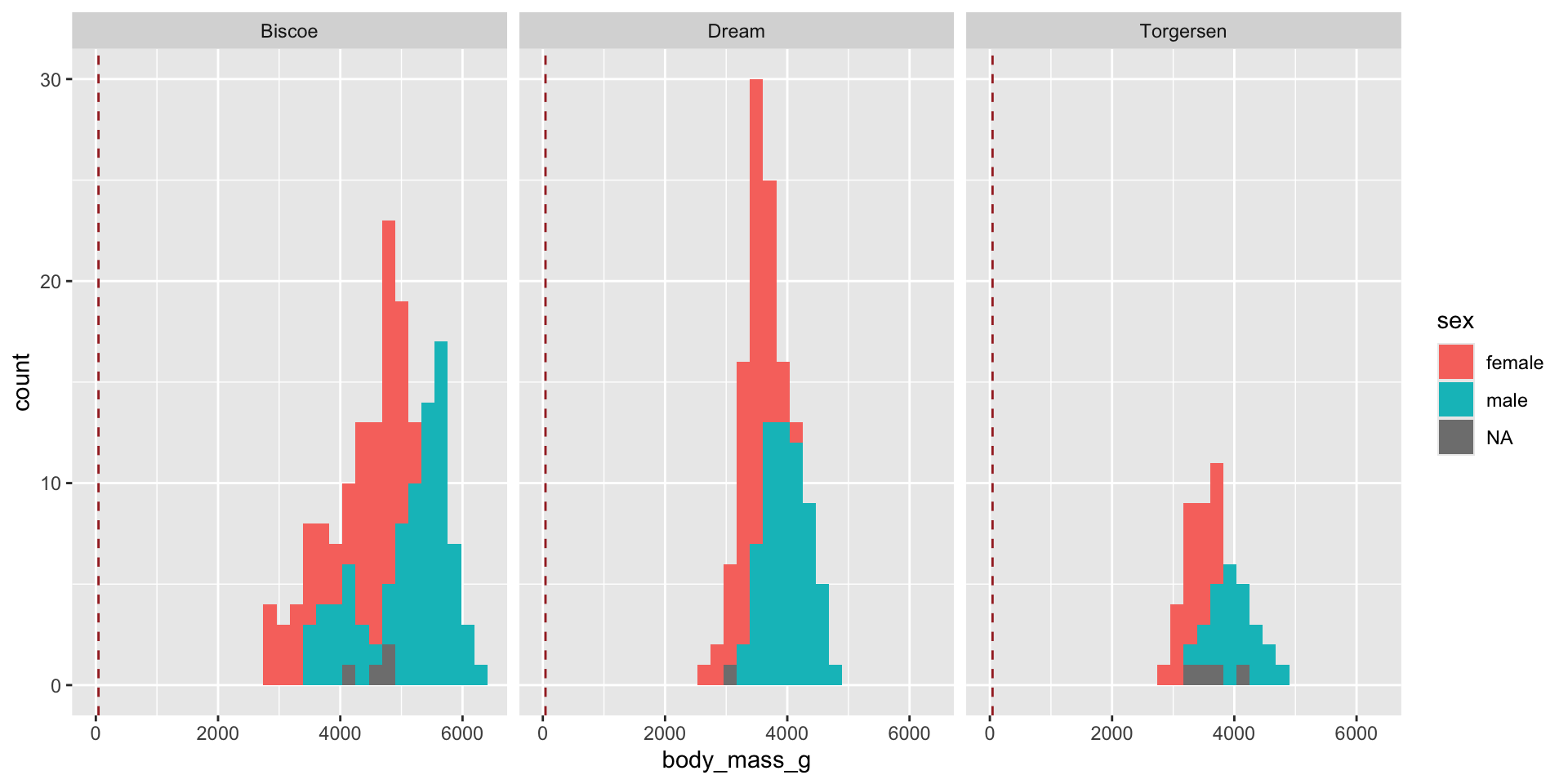
Create Histograms

To see the spread, center and shape of a numeric variable.

penguins |>
  ggplot() +
  geom_histogram(aes(x=body_mass_g))

Histograms

1. Make bins for the numbers
2. Counts the occurrence of a value within bins
3. The height is the number of counts.

We can adjust the bin or bin size.

Try one:

Copy some code above as a template and try to make a histogram of body_mass_g.

Add a vertical line at the mean() value, fill by sex and facet by island.

Answer:

Here is my solution to the problem on the previous slide.

mean_bill_len = mean(penguins$bill_length_mm, na.rm = TRUE)

penguins |>
  ggplot(aes(x = body_mass_g, fill = sex))+
  geom_histogram()+
  geom_vline(
    xintercept = mean_bill_len,
    color="brown",
    linetype="dashed")+
  facet_grid(~island)